HDMA
Data download and descriptions
This file provides more detailed description of the data and analysis products deposited on Zenodo at https://zenodo.org/communities/hdma, and demonstrates how to programmatically search for and download specific files.
- A description of all data types and the corresponding URL and DOI is provided in Table S14 of the manuscript
- This documentation explains data formats, but please see the Methods section of the manuscript for details on how these were generated or computed
Contents:
- Downloading data from Zenodo
- Fragment files and count matrices
- Seurat objects
- ArchR projects
- BPCells object
- ChromBPNet training regions
- Trained ChromBPNet models
- ChromBPNet mean contribution scores
- Bigwig tracks for observed and predicted accessibility and contrib. scores
- Motif lexicon and motifs per cell type
- Motif instances
- Genomic tracks on the WashU Genome Browser
- Processing raw anonymized data from SRA
Downloading data from Zenodo
Any records on Zenodo can be downloaded by navigating to the record URL provided in Table S14 and downloading from the webs.
Programmatic download
For programmatic access, we provide the following helper script for getting links to the latest version of all files in a set of Zenodo records, from the latest version of each record. This is useful since many of our data types are split across several depositions, and one may want to download several files or types of files across several depositions. We also provide some examples of how to download specific files across many depositions.
(Another option is the zenodo_get python package, which allows for downloading all data in a record, or fetching direct links to all files within a record, from the command line. Important note: for zenodo_get, the input must be one of the versioned DOIs for the record, not the record that resolves to the latest version. The latter is what is provided in Table S14.)
Helper script
We will use the following helper script, get_urls.py for getting links to all files in a set of Zenodo records,
from the latest version of each record.
# Input: space-separated Zenodo record IDs, from STDIN or passed as an argument
# Output: urls_record.txt with one line per record, corresponding to the URLs for the latest version
#         urls_file.txt with one line per file, corresponding to the direct download URL, for all files in all the input records
# Usage: $ python get_latest.py 15048277

import requests
import sys

def get_latest_zenodo_info(record_id):
	"""
	Fetches the latest DOI and HTML URL for a Zenodo record ID.

	Args:
		record_id (str): The Zenodo record ID.

	Returns:
		tuple: A tuple containing the latest DOI and HTML URL, or (None, None) on error.
	"""
	api_url = f"https://zenodo.org/api/records/{record_id}"

	try:
		response = requests.get(api_url)
		response.raise_for_status()  # Raise HTTPError for bad responses (4xx or 5xx)
		data = response.json()

		# Get the API URL of the latest version (which should be the same record)
		latest_html_url = data["links"]["self"]  # directly get the current record

		# Extract the DOI
		latest_doi = data["doi"]

		return latest_doi, latest_html_url

	except requests.exceptions.RequestException as e:
		return None, None
	except (KeyError, ValueError) as e:
		return None, None

def get_file_urls(record_id):
	"""
	Fetches file URLs for a given Zenodo record ID.

	Args:
		record_id (str): The Zenodo record ID.

	Returns:
		list: A list of file URLs, or an empty list on error.
	"""
	try:
		api_url = f"https://zenodo.org/api/records/{record_id}"
		response = requests.get(api_url)
		response.raise_for_status()
		data = response.json()
		file_urls = []
		for file_data in data['files']:
			fname = file_data['key']
			link = f"https://zenodo.org/record/{record_id}/files/{fname}"
			file_urls.append(link)
		return file_urls

	except requests.exceptions.RequestException as e:
		return []
	except (KeyError, ValueError) as e:
		return []

record_urls = []
file_urls_all = []
errors = []

# Determine source of record IDs (stdin or command line arguments)
record_ids = []
if not sys.stdin.isatty():
	record_ids = sys.stdin.read().strip().split()
else:
	record_ids = sys.argv[1:]

for record_id in record_ids:
	if not record_id:
		continue

  print(record_id)
	latest_doi, latest_html_url = get_latest_zenodo_info(record_id)
	if latest_doi and latest_html_url:
		record_urls.append(latest_html_url)

		latest_record_id = latest_html_url.split("/")[-1]  # Extract record ID from URL
		file_urls = get_file_urls(latest_record_id)
		file_urls_all.extend(file_urls)
	else:
		errors.append(f"Error processing record ID {record_id}")

if errors:
	for error in errors:
		print(error)
else:
	with open("urls_record.txt", "w") as record_file:
		for url in record_urls:
			record_file.write(url + "\n")

	with open("urls_file.txt", "w") as file_file:
		for url in file_urls_all:
			file_file.write(url + "\n")

	print("Record URLs written to urls_record.txt")
	print("File URLs written to urls_file.txt")
Example: get trained ChromBPNet models for Brain cell types
# list the data types on Zenodo from Table S14
cut -f 1 tables/table_s14.tsv | sort | uniq
# ArchR projects
# Bigwigs
# BPCells objects
# Cell metadata, caCREs, ChromBPNet training regions, instances, motif lexicon
# ChromBPNet counts mean contribution scores (h5)
# ChromBPNet models
# ChromBPNet models, and shared bias model
# data_type
# Fragments + count matrices
# Per-cluster TF-MoDISco motifs (h5)
# Seurat objects

# record IDs are in column 4 of Table S14, so we pipe those
# into our helper to get the URLs for the files from records containing ChromBPNet models
grep models tables/table_s14.tsv | cut -f 4 | tr '\n' ' ' | python get_urls.py
# Record URLs written to urls_record.txt
# File URLs written to urls_file.txt

# get the URLs for all Brain cell types
grep Brain urls_file.txt > urls_brain.txt

# download the Brain models
wget -i urls_brain.txt
for i in *.gz; do tar -xvf $i; done
Example: get the Seurat object for brain tissue
grep Seurat tables/table_s14.tsv | cut -f 4 | tr '\n' ' ' | python get_urls.py
# Record URLs written to urls_record.txt
# File URLs written to urls_file.txt

# get the URL for the Brain object
grep Brain urls_file.txt > urls_brain.txt

# download the Brain models
wget -i urls/brain_urls.txt
Example: get all fragment files
# get the records containing Fragments + Count Matrices
grep Fragments tables/table_s14.tsv | cut -f 4 | tr '\n' ' ' | python get_urls.py
# Record URLs written to urls_record.txt
# File URLs written to urls_file.txt

# get the URLs for all fragments and fragment index files
grep fragments urls_file.txt > urls_fragment.txt

# download the fragments files & index files
wget -i urls_fragment.txt
Example: get bigwigs for all immune cell types
# get the records containing Bigwigs
grep Bigwig tables/table_s14.tsv | cut -f 4 | tr '\n' ' ' | python get_urls.py

# preview the columns in Table S2
head -n2 tables/table_s2.tsv
# Cluster	organ	organ_code	cluster_id	compartment	L1_annot	L2_annot	L3_annot	dend_order	ncell	median_numi	median_ngene	median_nfrags	median_tss	median_frip	note	organ_color	compartment_color	Cluster_ChromBPNet
# LI_13	Liver	LI	13	epi	LI_13_cholangiocyte	Liver cholangiocyte	cholangiocyte	1	1004	1986	1462.5	7509.5	11.826	0.516103027	PKHD1 ANXA4 cholangiocyte (secretes bile)	#3b46a3	#11A579	Liver_c13

# get all cell types where compartment == "imm", extract the Cluster_ChromBPNet column value,
# and get the URLs matching those IDs
awk -F'\t' '$5 == "imm" { print $19 }' tables/table_s2.tsv | grep -f - urls_file.txt > urls_imm.txt

# download the bigwigs for immune cell types
wget -i urls_imm.txt
Fragment files and count matrices
One ATAC fragment file and tabix index per sample, named <sample>.fragments.tsv.gz and <sample>.fragments.tsv.gz.tbi. Genomic coordinates in fragment files are 0-based.
Three RNA count matrices files per sample in Matrix Market Exchange format:
<sample>.barcodes.tsv.gzcontains cell barcodes in the formatCL[cell library #]_[round 1 barcode plate position]+[round 2 barcode plate position]+[round 3 barcode plate position], e.g.CL131_C01+A01+A01.<sample>.features.tsv.gzcontains Ensembl gene IDs and the gene names<sample>.matrix.mtx.gzcontains the non-zero entries in the sparse matrix, with features and barcodes as rows and columns respectively
Seurat objects
One Seurat V4 object as a serialized RDS object per organ, named <organ>_RNA_obj_clustered_final.rds.
Objects contain the RNA data for all cells passing QC; ATAC data is not present in these objects.
The cell metadata (<object>@meta.data) contains sample information and cell annotations:
Samplecorresponds to the same column in Table S2annotv1corresponds tocompartmentin Table S2 with anorgan_codeprefixannotv2corresponds toL2_annotin Table S2 (in Table S2, it’s prefixed byorgan)
Each object contains 3 assays:
<object>@assays$RNA: UMI counts<object>@assays$SCT: SCTransformed UMI counts<object>@assays$decontX: decontX run on SCTransformed-UMI counts, to produce count matrices corrected for ambient RNA expression. This assay was used for visualization of gene expression throughout the paper.
e.g. in R:
# load object for Adrenal
adrenal <- readRDS("Adrenal_RNA_obj_clustered_final.rds")
adrenal@meta.data %>% tibble::glimpse()
# Rows: 2,883
# Columns: 25
# $ orig.ident          <chr> "CL131", "CL131", "CL131", "CL131", "CL131", "CL131", "CL131", "CL131"…
# $ nCount_RNA          <dbl> 10283, 22085, 17195, 12484, 10271, 10032, 15655, 11016, 18970, 4805, 4…
# $ nFeature_RNA        <int> 3453, 5526, 4864, 4014, 3876, 3645, 5096, 4483, 5039, 2340, 2365, 3250…
# $ percent.mt          <dbl> 0.009724788, 0.009055920, 0.000000000, 0.008010253, 0.009736150, 0.000…
# $ passfilter          <lgl> TRUE, TRUE, TRUE, TRUE, TRUE, TRUE, TRUE, TRUE, TRUE, TRUE, TRUE, TRUE…
# $ Sample              <chr> "T273_b16_Adr_PCW18", "T273_b16_Adr_PCW18", "T273_b16_Adr_PCW18", "T27…
# $ sex                 <chr> "M", "M", "M", "M", "M", "M", "M", "M", "M", "M", "M", "M", "M", "M", …
# $ PCW                 <chr> "PCW18", "PCW18", "PCW18", "PCW18", "PCW18", "PCW18", "PCW18", "PCW18"…
# $ PCD                 <chr> "PCD126", "PCD126", "PCD126", "PCD126", "PCD126", "PCD126", "PCD126", …
# $ age                 <chr> "PCW18", "PCW18", "PCW18", "PCW18", "PCW18", "PCW18", "PCW18", "PCW18"…
# $ S.Score             <dbl> -0.042831648, -0.091017252, -0.075550268, -0.143961927, -0.008328376, …
# $ G2M.Score           <dbl> -0.053519769, -0.408871745, -0.230472517, -0.005143041, -0.092735455, …
# $ Phase               <chr> "G1", "G1", "G1", "G1", "G1", "S", "G1", "S", "G1", "S", "G1", "G1", "…
# $ nCount_SCT          <dbl> 8086, 7344, 7914, 8205, 8123, 8090, 8251, 8203, 7772, 6688, 6548, 8001…
# $ nFeature_SCT        <int> 3422, 3027, 3561, 3788, 3833, 3614, 4197, 4409, 3366, 2327, 2365, 3228…
# $ SCT_snn_res.0.3     <fct> 2, 2, 2, 2, 2, 2, 4, 5, 2, 2, 5, 2, 2, 5, 2, 6, 2, 2, 2, 2, 2, 6, 2, 2…
# $ seurat_clusters     <fct> 2, 2, 2, 2, 2, 2, 4, 5, 2, 2, 5, 2, 2, 5, 2, 6, 2, 2, 2, 2, 2, 6, 2, 2…
# $ Clusters            <fct> 2, 2, 2, 2, 2, 2, 4, 5, 2, 2, 5, 2, 2, 5, 2, 6, 2, 2, 2, 2, 2, 6, 2, 2…
# $ estConp             <dbl> 0.30891153, 0.13286947, 0.17151322, 0.24562908, 0.51484749, 0.33882811…
# $ nCount_decontX      <dbl> 6026, 6775, 7050, 6733, 3929, 5714, 2715, 3481, 7371, 4119, 5477, 6580…
# $ nFeature_decontX    <int> 3159, 2977, 3473, 3554, 2418, 3257, 1841, 2427, 3329, 2003, 2299, 3093…
# $ decontX_snn_res.0.3 <fct> 2, 2, 2, 2, 2, 2, 4, 5, 2, 2, 5, 2, 2, 5, 2, 6, 2, 2, 2, 2, 2, 6, 2, 2…
# $ annotv1             <chr> "AG_epi", "AG_epi", "AG_epi", "AG_epi", "AG_epi", "AG_epi", "AG_epi", …
# $ keepcell            <lgl> TRUE, TRUE, TRUE, TRUE, TRUE, TRUE, TRUE, TRUE, TRUE, TRUE, TRUE, TRUE…
# $ annotv2             <chr> "adrenal cortex", "adrenal cortex", "adrenal cortex", "adrenal cortex"…
ArchR projects
One zipped folder per organ containing the ArchR project (Save-ArchR-Project.rds) and all associated files, named <organ>_ATAC_obj_clustered_peaks_final_decontx.zip.
See the ArchR documentation on loading projects here.
ArchR projects contain the ATAC data for all cells passing QC; RNA data is also appended to these projects.
The cell metadata (getCellColData(<project>)) contains sample information and cell annotations:
Samplecorresponds to the same column in Table S2RNA_Clusterscorresponds to the RNA-derived cell clusters stored incluster_idin Table S2, with a “c” letter prefixRNA_NamedCluster_L1corresponds tocompartmentin Table S2 with anorgan_codeprefixRNA_NamedCluster_L2corresponds toL2_annotin Table S2 (in Table S2, it’s prefixed byorgan)ATAC_Clustersare clusters identified using ATAC Tile data only (Iterative LSI transformed Tile Matrix), not used in manuscriptATAC_Clusters_Peakare clusters identified using ATAC Peak data only (Iterative LSI transformed Peak Matrix), not used in manuscript
Each project contains 5 matrices:
GeneExpressionMatrix: counts (not log normalized) from thedecontXassay of the organ’s Seurat objectGeneScoreMatrix,MotifMatrix,PeakMatrixandTileMatrixconstructed using standard ArchR processing workflows
e.g. in R:
# load project for Adrenal
adrenal <- loadArchRProject("ATAC_obj_clustered_peaks_final_decontx/")
adrenal
#
#            ___      .______        ______  __    __  .______
#           /   \     |   _  \      /      ||  |  |  | |   _  \
#          /  ^  \    |  |_)  |    |  ,----'|  |__|  | |  |_)  |
#         /  /_\  \   |      /     |  |     |   __   | |      /
#        /  _____  \  |  |\  \\___ |  `----.|  |  |  | |  |\  \\___.
#       /__/     \__\ | _| `._____| \______||__|  |__| | _| `._____|
#
# class: ArchRProject
# outputDirectory: /path/to/Adrenal/atac_preprocess_output/ATAC_obj_clustered_peaks_final_decontx
# samples(4): T318_b16_Adr_PCW21 T40_b16_Adr_PCW17 T273_b16_Adr_PCW18 T390_b16_Adr_PCW13
# sampleColData names(1): ArrowFiles
# cellColData names(26): Sample TSSEnrichment ... FRIP ATAC_Clusters_Peak
# numberOfCells(1): 2883
# medianTSS(1): 9.872
# medianFrags(1): 5437

getAvailableMatrices(adrenal)
# [1] "GeneExpressionMatrix" "GeneScoreMatrix"      "MotifMatrix"          "PeakMatrix"           "TileMatrix"

getCellColData(adrenal) %>% tibble::glimpse()
# Formal class 'DFrame' [package "S4Vectors"] with 6 slots
#   ..@ rownames       : chr [1:2883] "T318_b16_Adr_PCW21#CL131_E01+H09+A09" "T318_b16_Adr_PCW21#CL131_E03+G11+A10" "T318_b16_Adr_PCW21#CL131_E05+C09+A09" "T318_b16_Adr_PCW21#CL131_E07+B08+A08" ...
#   ..@ nrows          : int 2883
#   ..@ listData       :List of 26
#   .. ..$ Sample              : chr [1:2883] "T318_b16_Adr_PCW21" "T318_b16_Adr_PCW21" "T318_b16_Adr_PCW21" "T318_b16_Adr_PCW21" ...
#   .. ..$ TSSEnrichment       : num [1:2883] 10.75 10.35 9.33 9.3 9.38 ...
#   .. ..$ ReadsInTSS          : num [1:2883] 31418 27337 20101 19281 20050 ...
#   .. ..$ ReadsInPromoter     : num [1:2883] 32813 29854 22357 21415 21334 ...
#   .. ..$ ReadsInBlacklist    : num [1:2883] 1012 871 764 539 537 ...
#   .. ..$ PromoterRatio       : num [1:2883] 0.168 0.191 0.161 0.176 0.178 ...
#   .. ..$ PassQC              : num [1:2883] 1 1 1 1 1 1 1 1 1 1 ...
#   .. ..$ NucleosomeRatio     : num [1:2883] 2.15 1.71 1.82 1.82 1.81 ...
#   .. ..$ nMultiFrags         : num [1:2883] 43118 30620 27556 24036 23236 ...
#   .. ..$ nMonoFrags          : num [1:2883] 31014 28823 24574 21584 21330 ...
#   .. ..$ nFrags              : num [1:2883] 97567 78222 69279 60787 59842 ...
#   .. ..$ nDiFrags            : num [1:2883] 23435 18779 17149 15167 15276 ...
#   .. ..$ BlacklistRatio      : num [1:2883] 0.00519 0.00557 0.00551 0.00443 0.00449 ...
#   .. ..$ age                 : chr [1:2883] "PCW21" "PCW21" "PCW21" "PCW21" ...
#   .. ..$ RNA_Clusters        : chr [1:2883] "c0" "c5" "c0" "c3" ...
#   .. ..$ Gex_nUMI            : num [1:2883] 6234 2195 6290 6186 6023 ...
#   .. ..$ Gex_nGenes          : num [1:2883] 2707 1533 2861 2640 2806 ...
#   .. ..$ Gex_MitoRatio       : num [1:2883] 0.00353 0.00273 0.00366 0.00388 0.00349 ...
#   .. ..$ Gex_RiboRatio       : num [1:2883] 0.00417 0.00273 0.00302 0.00453 0.00432 ...
#   .. ..$ ATAC_Clusters       : chr [1:2883] "C4" "C5" "C4" "C4" ...
#   .. ..$ RNA_NamedCluster_L1 : chr [1:2883] "AG_epi" "AG_end" "AG_epi" "AG_epi" ...
#   .. ..$ RNA_NamedCluster_L1b: chr [1:2883] "AG_epi1" "AG_end" "AG_epi1" "AG_epi4" ...
#   .. ..$ RNA_NamedCluster_L2 : chr [1:2883] "adrenal cortex" "endothelial" "adrenal cortex" "adrenal cortex" ...
#   .. ..$ ReadsInPeaks        : num [1:2883] 54467 44226 37898 35782 36616 ...
#   .. ..$ FRIP                : num [1:2883] 0.28 0.283 0.274 0.295 0.306 ...
#   .. ..$ ATAC_Clusters_Peak  : chr [1:2883] "C2" "C3" "C2" "C2" ...
#   ..@ elementType    : chr "ANY"
#   ..@ elementMetadata: NULL
#   ..@ metadata       : list()
BPCells object
A BPCells object containing fragment files, count matrices, cell metadata, ABC loops
per cluster, and motif instances per cluster is provided at ![]() :
:
cell_metadata: the per cell metadatafrags: path to unzipped folder of ATAC fragments ‘ATAC_merged’rna: path to unzipped folder of unnormalized decontX’ed RNA count matrices ‘RNA_merged’rna_raw: path to unzipped folder of unnormalized raw RNA count matrices ‘RNA_raw_merged’transcripts: GENCODE human release 42 gene annotationloops_p2g: Peak2Gene loops per organ or globally across organsloops_abc: ABC loops per L1 clusterpeaks: HDMA global caCREshits: all annotated motif instances called using ChromBPNet
The BPCells object was produced by the script code/05-misc/01-bp_cells_create_obj.R.
The BPCells object was primarily used for efficient plotting and visualization of genomic
loci. See our notebook with examples for plotting using the BPCells object
at code/05-misc/02-bp_cells_plotting_examples.Rmd (html).
NOTE: the BPCells package uses on-disk storage, so the fragment files and count matrices in the RDS object only point to the path where the files are stored, and it’s important to modify those paths when the folders are moved or downloading this object locally. See the BPCells paper (Parks & Greenleaf, biorxiv, 2025) for more details on the compression and storage in BPCells objects.
ChromBPNet training regions
The peak and background (non-peak) regions used to train the ChromBPNet models
are provided as a single tar archive, all_training_regions.tar.gz, in the Zenodo
depo ![]() .
These are the per-cell type peak sets used as input for training (and used, for example,
as the input peaks for the g-chromVAR analysis).
.
These are the per-cell type peak sets used as input for training (and used, for example,
as the input peaks for the g-chromVAR analysis).
The archive extracts to a directory 4-peaks/all/ containing, for each cluster
(named using the Cluster_ChromBPNet cluster ID from Table S2):
<cluster>__peaks_bpnet.bed: the peak regions used to train ChromBPNet, 1,000 bp windows centered on the peak summit<cluster>__nonpeaks_fold_<0-4>.bed: the GC-matched background (non-peak) regions, provided per training fold (fold_0throughfold_4)
The peak BED files have 10 columns following the ChromBPNet convention, where the
first three are chr, start, end (a 1,000 bp window), and the final column is
the summit offset relative to the region start (i.e. 500):
$ wget https://zenodo.org/record/17427146/files/all_training_regions.tar.gz
$ tar -xvf all_training_regions.tar.gz
$ cd 4-peaks/all
$ ls Muscle_c6*
Muscle_c6__nonpeaks_fold_0.bed  Muscle_c6__nonpeaks_fold_2.bed  Muscle_c6__nonpeaks_fold_4.bed
Muscle_c6__nonpeaks_fold_1.bed  Muscle_c6__nonpeaks_fold_3.bed  Muscle_c6__peaks_bpnet.bed
$ head Muscle_c6__peaks_bpnet.bed
chr1	183987	184987	.	.	.	.	.	.	500
chr1	191014	192014	.	.	.	.	.	.	500
chr1	191356	192356	.	.	.	.	.	.	500
chr1	267506	268506	.	.	.	.	.	.	500
chr1	585697	586697	.	.	.	.	.	.	500
chr1	777915	778915	.	.	.	.	.	.	500
chr1	778232	779232	.	.	.	.	.	.	500
chr1	778677	779677	.	.	.	.	.	.	500
chr1	816861	817861	.	.	.	.	.	.	500
chr1	817597	818597	.	.	.	.	.	.	500
Trained ChromBPNet models
One tar archive per cluster, using the Cluster_ChromBPNet cluster ID from Table S2, named <cluster>.gz.
Only models which passed QC and which were used for downstream analysis are provided, thus there
are models for 189 cell types.
The bias model was trained on Heart_c0 fold_0, and the bias model was used for training all ChromBPNet models.
The tar archive for each cluster can be extracted with tar -xvf and contains 15 models as weights saved as H5 files
named <cluster>__<fold>__<model>.h5:
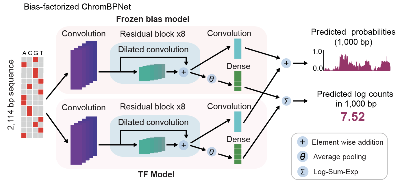
<fold>indicates the chromosome fold<model>indicates the model type:bias_model_scaled: the final bias model used for this cell type on this fold, resulting from the scaling of the counts output of the input bias model (which is shared across cell types), to account for differences in coverage between the bias model training dataset and the current cell typechrombpnet_nobias: the submodel which predicts residual accessibility not explained by Tn5 sequence bias, a.k.a. the bias-corrected model. This model is used throughout all downstream analysis in the paper. Use this model to obtain bias-corrected accessibility predictions for genomic sequences.chrombpnet: the full accessibility model, which is the combination ofbias_model_scaledandchrombnet_nobias, and predicts the observed accessibility (resulting from both Tn5 sequence bias and other DNA binding events).
From the model schematic below from the ChromBPNet paper (Pampari, Scherbina et al, biorxiv, 2024),
bias_model_scaled is the “Frozen bias model”, chrombpnet_nobias is the “TF model”, and chrombpnet is
the total model with both submodels together.
We show how to load and use trained ChromBPNet models in the tutorial at code/05-misc/04-ChromBPNet_use_cases.ipnyb (html).
ChromBPNet mean contribution scores
One H5 file per cluster, using the Cluster_ChromBPNet cluster ID from Table S2, named <cluster>__average_shaps.counts.h5.
Bigwig tracks for observed and predicted accessibility and contrib. scores
One zipped directory per cluster, using the Cluster_ChromBPNet cluster ID from Table S2, named <cluster>__bigwigs.gz.
Each directory contains the following genomic tracks:
<cluster>__obs_pval_signal.bw: Macs2 p-value signal track for observed accessibility<cluster>__mean_pred_corrected.bw: bias-corrected accessibility predicted by ChromBPNet (predictions are averaged across five folds)<cluster>__mean_counts_contribs.bw: base-resolution contribution scores for the counts head of ChromBPNet as computed by DeepLIFT (contribution scores are averaged across five folds). Scores are computed for input regions, i.e. 2,114 bp regions where the central 1,000 bp corresponds to an input peak region
NOTE: for viewing contribution scores in a genome browser, we recommend loading these bigwgigs as dynseq tracks in the WashU or UCSC genome browsers, which render the nucleotide character (A/C/G/T) at each position, where character height is proportional to the contribution score at that position. When zoomed out, the tracks appear as regular bigwigs. See the dynseq paper (Nair et al, Nature Genetics, 2022) for more details and documentation.
Motif lexicon and motifs per cell type
Motifs per cell type
We also provide the 6,362 motifs learned with TF-MoDISco in each cell type, in the Zenodo depo ![]() :
:
- tar archive
all_modisco_outputs.tar.gzcontaining:- one h5 file produced by TF-MoDISco per cell type, named
<cluster>__counts_modisco_output.h5using theCluster_ChromBPNetcluster ID from Table S2 containing the motifs CWMs as matrices - the TF-MoDISco report,
<cluster>__counts_modisco_reportusing theCluster_ChromBPNetcluster ID from Table S2, a directory containing:trimmed_logos: CWM logos (forward and reverse) for all TF-MoDISco motifs discovered in that model, as PNGsmotifs.html: HTML file corresponding to the TF-MoDISco report, which depends on the logos in the directory, and can be viewed in a browser. Each row corresponds to one de novo CWM, and indicates the number of seqlets associated with that CWM, the forward and reverse logos, and the best matches to an external motif database.
- one h5 file produced by TF-MoDISco per cell type, named
- one TSV file,
merged_modisco_patterns_map.tsv, with a header and 6,362 rows: for every motif learned in every cell type, which maps it to the aggregated compendium motifs. The columnmerged_patternmatches the column of the same name in Table S6.
Following the documentation from tf-modiscolite, the h5 files have this format:
pos_patterns/
    pattern_0/
        sequence: [...]
        contrib_scores: [...]
        hypothetical_contribs: [...]
        seqlets/
            n_seqlets: [...]
            start: [...]
            end: [...]
            example_idx: [...]
            is_revcomp: [...]
            sequence: [...]
            contrib_scores: [...]
            hypothetical_contribs: [...]
        subpattern_0/
            ...
    pattern_1/
        ...
    ...
neg_patterns/
    pattern_0/
        ...
    pattern_1/
        ...
    ...
In the TF-MoDISco terminology, “seqlets” are short genomic loci which are contiguous regions of high-contribution nucleotides, and they are clustered into “patterns”, or motifs.
pos_patternscontain the positive motifs (which positively contribute to accessibility)neg_patternscontain the negative motifs (which negatively contribute to accessibility)- For each pattern:
seqletscontains the coordinates of loci used to construct the motif relative to the input peaks:example_idxgives the index of the input locusstartgives the start of seqlet within the input locusendgives the end of the seqlet within the input locus
sequencecontains the position-frequency matrix (PFM) representation for each motif, in the form of probabilities which sum to 1 across nucleotides, per positioncontrib_scorescontains the contribution-weight matrix (CWM) representation for each motif, computed as the average contribution scores across aligned seqlets clustered into the motif patternhypothetical_contribscontains the hypothetical contribution-weight matrix (hCWM) representation for each motif, computed from the hypothetical contribution scores across seqlets. These are the computed scores for all four possible nucleotides at each sequence, not just the observed nucleotide. See tfmodisco/issues/5 for more discussion on the purpose of hypothetical contributions.
The h5 file can be loaded e.g. in python:
import h5py
modisco_obj = h5py.File("Adrenal_c0__counts_modisco_output.h5")
modisco_obj
# <HDF5 file "Adrenal_c0__counts_modisco_output.h5" (mode r)>
modisco_obj['pos_patterns']
# <HDF5 group "/pos_patterns" (39 members)>
modisco_obj['neg_patterns']
# <HDF5 group "/neg_patterns" (3 members)>
The merged_modisco_patterns_map.tsv can be used to match per-cell type motifs to their motif cluster in the lexicon:
head merged_modisco_patterns_map.tsv
merged_pattern	component_celltype	pattern_class	pattern	n_seqlets	component_pattern
neg.Average_12__merged_pattern_0	Spleen_c5	neg_patterns	pattern_0	88	Spleen_c5__neg_patterns.pattern_0
neg.Average_12__merged_pattern_0	Spleen_c0	neg_patterns	pattern_0	461	Spleen_c0__neg_patterns.pattern_0
neg.Average_12__merged_pattern_0	Skin_c5	neg_patterns	pattern_0	302	Skin_c5__neg_patterns.pattern_0
neg.Average_12__merged_pattern_0	Heart_c13	neg_patterns	pattern_0	128	Heart_c13__neg_patterns.pattern_0
neg.Average_12__merged_pattern_0	Skin_c7	neg_patterns	pattern_0	708	Skin_c7__neg_patterns.pattern_0
neg.Average_12__merged_pattern_0	Heart_c5	neg_patterns	pattern_0	47	Heart_c5__neg_patterns.pattern_0
neg.Average_12__merged_pattern_0	Heart_c4	neg_patterns	pattern_0	41	Heart_c4__neg_patterns.pattern_0
neg.Average_12__merged_pattern_0	Skin_c9	neg_patterns	pattern_0	335	Skin_c9__neg_patterns.pattern_0
neg.Average_12__merged_pattern_0	Heart_c2	neg_patterns	pattern_0	93	Heart_c2__neg_patterns.pattern_0
Motif lexicon
To generate the motif lexicon (also referred to as motif compendium in the code base), the 6,362 motifs discovered in each of the 189 cell types (using TF-MoDISco) were aggregated together and subjected to QC. This resulted in a total of 508 motifs.
Table S6 contains a summary table of the motif lexicon, one row per motif, along with its granular and broad annotations. The motifs can be explored interactively along with summary stats across tisuses and best matches to know motifs here: https://greenleaflab.github.io/HDMA/MOTIFS.html
We provide the following resources for the motif lexicon in the Zenodo depo ![]() :
:
- h5 file in the TF-MoDISco format containing motif CWMs as matrices (
motif_compendium.modisco_object.h5) - PPMs in MEME format:
motif_compendium.PPM.memedb.txt - PPMs of trimmed motifs in MEME format:
motif_compendium.trimmed.PPM.memedb.txt - PNG images of forward and reverse-complemented CWM logos:
denovo_motifs_508_cwm_images.gz
To match the motifs in the lexicon h5 object to their names, use column R, “merged_pattern”, in Table S6, which corresponds to the keys in the object.
Motif instances
The genomic tracks of annotated predictive motif instances in peaks are provided for each cluster as a zipped file motif_instances.gz in the Zenodo depo ![]()
For every cluster, there are three files.
A BED file: <cluster>__instances.bed.gz>, with the columns chr, start, end, motif_name, hit_score, strand, pattern_class:
$ zcat Adrenal_c0__instances.bed.gz | head
chr1	10175	10180	456|ZEB/SNAI	888.5867	-	neg_patterns
chr1	10566	10575	436|SP/KLF	931.89967	+	pos_patterns
chr1	181096	181105	436|SP/KLF	933.10714	+	pos_patterns
chr1	181151	181161	400|NRF1	966.9898999999999	-	pos_patterns
chr1	181180	181190	400|NRF1	962.5238	-	pos_patterns
chr1	181209	181219	400|NRF1	951.84535	-	pos_patterns
chr1	181238	181248	400|NRF1	949.1391	-	pos_patterns
chr1	181267	181277	400|NRF1	944.7280999999999	-	pos_patterns
chr1	181296	181306	400|NRF1	934.34006	-	pos_patterns
chr1	181325	181335	400|NRF1	930.62365	-	pos_patterns
A TSV file: <cluster>__instances.annotated.tsv.gz, with a more extended set of information (including hit scores and genomic annotaitons) per motif instance:
$ zcat Adrenal_c0__instances.annotated.tsv.gz | head
seqnames	start	end	width	strand	start_untrimmed	end_untrimmed	motif_name	source	hit_coefficient	hit_correlation	hit_importance	peak_name	peak_id	motif_name_unlabeled	pattern_class	distToGeneStart	nearestGene	peakType	distToTSS	nearestTSS	GC	N	distToPeakSummit
chr1	10175	10180	5	-	10158	10188	456|ZEB/SNAI	2	1.1400998	0.8885867	0.009292185	NA	0	neg_patterns.neg.Average_12__merged_pattern_0	neg_patterns	1690	DDX11L1	Promoter	1690	ENST00000456328.2	0.4	0	71
chr1	10566	10575	9	+	10560	10590	436|SP/KLF	2	9.525877	0.93189967	0.02702999	NA	0	pos_patterns.pos.Average_212__merged_pattern_0	pos_patterns	1297	DDX11L1	Promoter	1297	ENST00000456328.2	0.8889	0	464
chr1	181096	181105	9	+	181090	181120	436|SP/KLF	1	1.8184662	0.93310714	0.0265913	NA	1	pos_patterns.pos.Average_212__merged_pattern_0	pos_patterns	1594	DDX11L17	Promoter	1594	ENST00000624431.2	0.8889	0	393
chr1	181151	181161	10	-	181138	181168	400|NRF1	2	8.63048	0.9669899	0.05363989	NA	1	pos_patterns.pos.Average_159__merged_pattern_0	pos_patterns	1539	DDX11L17	Promoter	1539	ENST00000624431.2	0.9	0	338
chr1	181180	181190	10	-	181167	181197	400|NRF1	2	4.2169023	0.9625238	0.038315773	NA	1	pos_patterns.pos.Average_159__merged_pattern_0	pos_patterns	1510	DDX11L17	Promoter	1510	ENST00000624431.2	0.9	0	309
chr1	181209	181219	10	-	181196	181226	400|NRF1	2	2.505722	0.95184535	0.03131914	NA	1	pos_patterns.pos.Average_159__merged_pattern_0	pos_patterns	1481	DDX11L17	Promoter	1481	ENST00000624431.2	0.9	0	280
chr1	181238	181248	10	-	181225	181255	400|NRF1	2	2.895874	0.9491391	0.036172867	NA	1	pos_patterns.pos.Average_159__merged_pattern_0	pos_patterns	1452	DDX11L17	Promoter	1452	ENST00000624431.2	0.9	0	251
chr1	181267	181277	10	-	181254	181284	400|NRF1	2	1.5476482	0.9447281	0.026664732	NA	1	pos_patterns.pos.Average_159__merged_pattern_0	pos_patterns	1423	DDX11L17	Promoter	1423	ENST00000624431.2	0.9	0	222
chr1	181296	181306	10	-	181283	181313	400|NRF1	2	1.0276077	0.93434006	0.023554802	NA	1	pos_patterns.pos.Average_159__merged_pattern_0	pos_patterns	1394	DDX11L17	Promoter	1394	ENST00000624431.2	0.9	0	193
Genomic tracks on the WashU Genome Browser
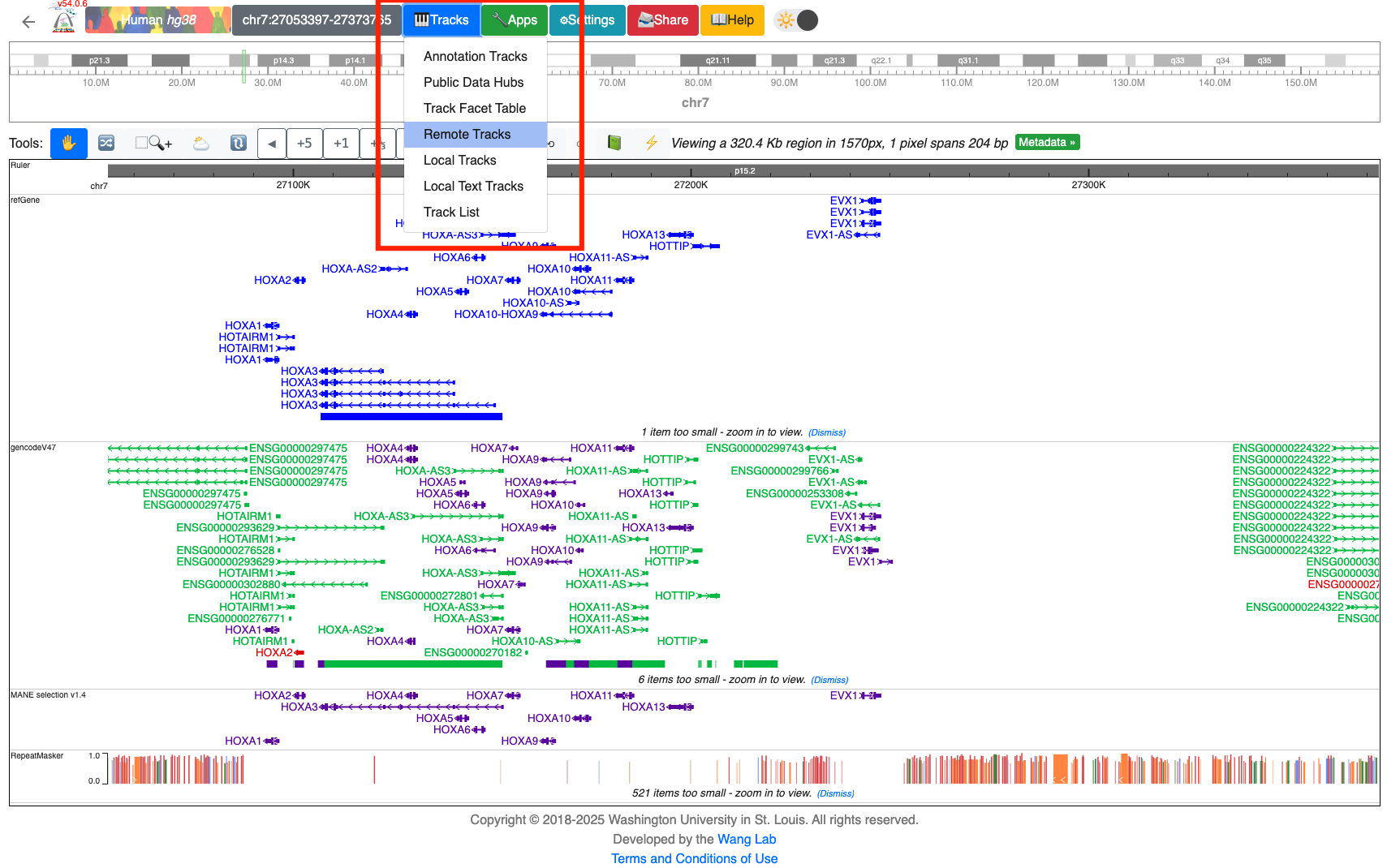
For easy interactive visualization, all genomic tracks can be loaded on the WashU Genome Browser using this link: https://epigenomegateway.wustl.edu/browser2022/?genome=hg38&hub=https://human-dev-multiome-atlas.s3.amazonaws.com/tracks/HDMA_trackhub.json.
For instructions on loading tracks, see below:
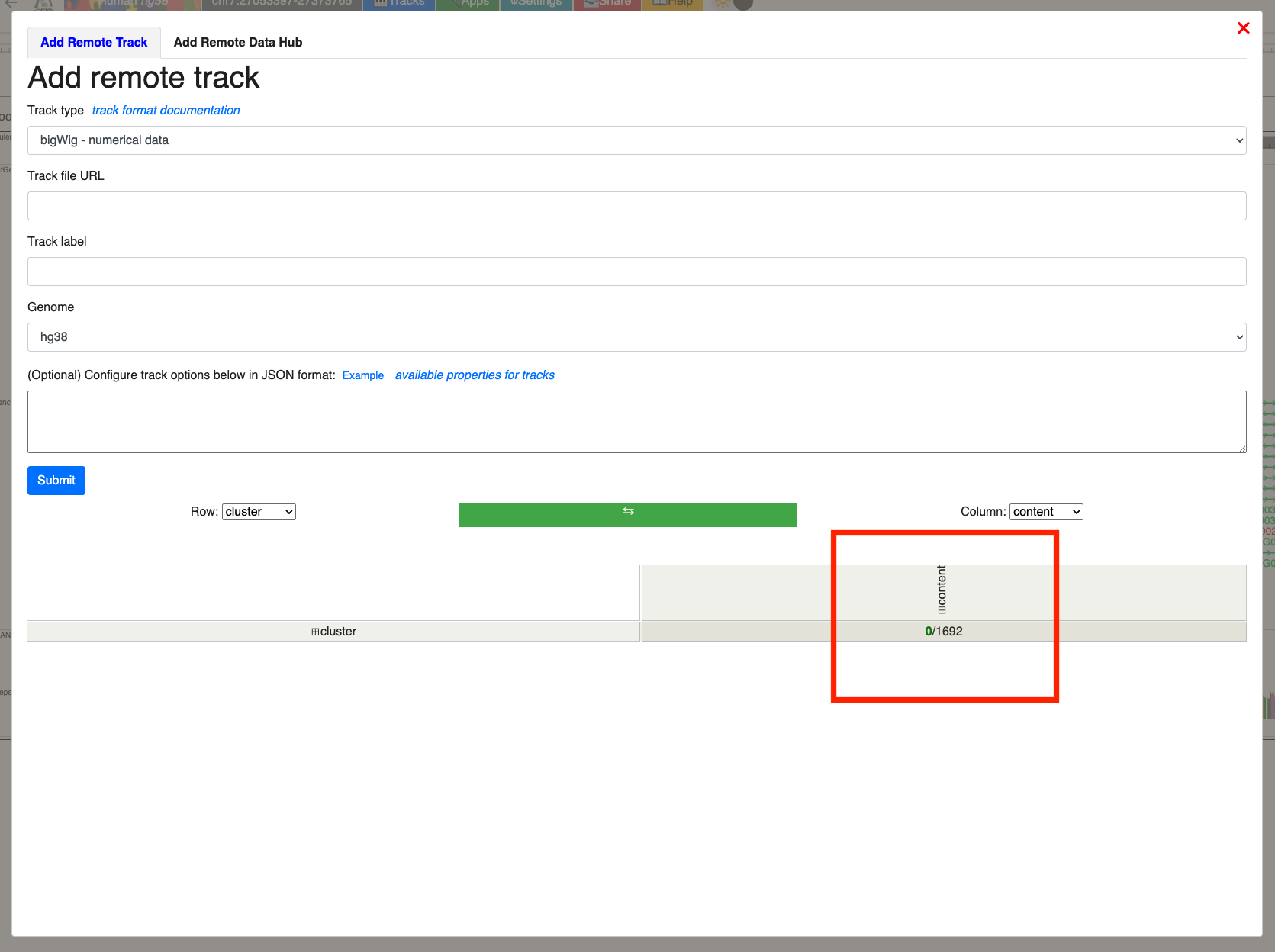
- Go to Tracks > Remote tracks:
- Click to expand the content:
- Use the track table to load cell types or tracks of interest:
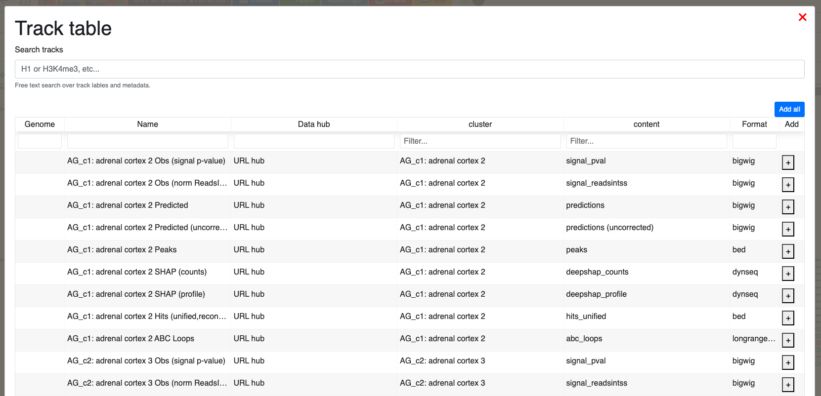
For each cluster, the following tracks are available:
signal_pval: Macs2 p-value signal track for observed accessibilitypredictions: bias-corrected accessibility predicted by ChromBPNet (predictions are averaged across five folds)predictions (uncorrected): uncorrected accessibility predicted by ChromBPNet (predictions are averaged across five folds)peaks: input regions for training ChromBPNet models (1,000 bp peaks centered at peak summits)deepshap_counts: base-resolution contribution scores for the counts head of ChromBPNet as computed by DeepLIFT (contribution scores are averaged across five folds). Scores are computed for input regions, i.e. 2,114 bp regions where the central 1,000 bp corresponds to an input peak regionhits_unified: BED files of annotated predictive motif instances identified using ChromBPNet modelling and Fi-NeMoabc_loops: ABC-loops inlongrangeformat
Processing raw anonymized data from SRA
HDMA anonymized raw data has been deposited to SRA under PRJNA1402391 in anonymized form: cell, sublibrary, and sample barcodes are preserved, but the read sequences were replaced with the corresponding reference genomic sequence (using BAMboozle). These anonymized FASTQs can be processed back into per-sample fragment files and count matrices using a dedicated branch of the SHARE-seq pipeline.
Pipeline overview
We have drafted some adaptations to our original SHARE-seq processing pipeline on the process-anonymize branch of
the GreenleafLab/shareseq-pipeline repo.
This chains three Snakemake workflows (see the branch
README
and example config
runs/share_sra_demo.yaml):
prep_sra.smk— downloads fastqs for each SRR declared in the run config intodata_dir, reconstructing the expected read header@<read> 1:N:0:<I1>+<I2>expected by our SHARE-seq pipeline. Outputs are named{ATAC|RNA}_{SampleID}_anon_{R1|R2}.fastq.gz. Skipped automatically when no SRRs are declared (i.e. FASTQs already at the expected paths if you downloaded them separately).ingest_anonymized.smk— splits each per-sample anonymized FASTQ back into per-sublibrary files (.fastq.zst) by matching read 2’s I2 index against the sublibrary→I2 map with 1 bp mismatch tolerance (mirroringbcl2fastq), then counts reads.shareseq.smk— standard SHARE-seq processing: matches the Round1+2+3 cell barcode, assigns each cell to a sample using the BC1 regex, aligns with bowtie2 (ATAC) / STAR (RNA), and writes per-sample outputs.
Expected outputs (under output_dir): ATAC/samples/<sample>.fragments.tsv.gz,
RNA/samples/<sample>.{matrix.mtx,barcodes.tsv,features.tsv}.gz, and QC JSONs
under {ATAC,RNA}/samples/. The cell barcode names
(CL{N}_BC1+BC2+BC3) match the published Seurat / ArchR objects other cell metadata
provided with the publication, so cells can be joined directly back to the published
metadata by cell barcode string.
Required inputs per batch
To configure a run (runs/<batch>.yaml), you need:
- Genome references — bowtie2 + STAR indexes, GENCODE GTF, hg38 FASTA.
Consult
scripts/references/prep_genome.sh hg38. - SRR accessions per sample, per assay — for
prep_sra.smkto fetch the anonymized FASTQs. See the SRA deposition PRJNA1402391. - Sample → Round1 BC1 regex and sublibrary (CL) → I2 index map — the same demultiplexing parameters used when the data was originally generated. These are provided in this repo (see below).
Demultiplexing parameter tables
The Round1 BC1 and CL→I2 index mappings for every batch in HDMA are
provided as two TSVs under
code/01-preprocessing/01-snakemake/,
alongside the original per-batch Snakemake configs they were derived from
(b{N}_<organ>.yaml):
sample_barcodes.tsv— one row per (organ, sample), columns:Organ,SampleName,SampleBarcodePattern. Use to populate thesamples:block of the run config. The 96 Round1 positions must be covered exactly once across all entries within a batch;dummyplaceholder rows exist for batches where a row was unassigned and must be retained verbatim.sublibrary_indices.tsv— one row per (organ, sequencing run, modality, sublibrary), columns:Organ,Modality(ATAC/RNA),Index(alwaysI2),Sublibrary(CL{N}),IndexSequence(8 bp). Use to populate thesublibraries: {ATAC: {...}, RNA: {...}}block of the run config.
Note on the Organ column. Organ groups entries by the processing batch,
not the biological tissue. Most batches map 1:1 to a single organ name (e.g.
Heart, Liver), but Lung was processed in two separate batches and is tagged
Lung_b12 and Lung_b18. Filter on the
exact Organ value when extracting a batch — substring-matching on tissue
names will collide (e.g. grep Lung returns both b12 and b18, and grep Spleen
returns both AdrenalThyroidSpleen and SpleenThymus).