Counts
This vignette covers the correct format for storing fragment counts for use in chromVAR.
library(chromVAR)
library(SummarizedExperiment)
library(Matrix)
chromVAR’s method for getting fragment counts
chromVAR includes a function getCounts for reading in fragment counts from bam or bed files.
peakfile <- system.file("extdata/test_bed.txt", package = "chromVAR")
peaks <- getPeaks(peakfile, sort_peaks = TRUE)
## Peaks sortedbamfile <- system.file("extdata/test_RG.bam", package = "chromVAR")
fragment_counts <- getCounts(bamfile,
peaks,
paired = TRUE,
by_rg = TRUE,
format = "bam",
colData = DataFrame(celltype = "GM"))## Reading in file: /home/travis/R/Library/chromVAR/extdata/test_RG.bam## Warning in doTryCatch(return(expr), name, parentenv, handler): length of
## NULL cannot be changedPaired vs single end data
The paired argument should be set based on whether the data is paired end. With paired end data, fragments are counted once if either or both ends of the fragment map to a peak. For single end data, a fragment is counted if the 5’ end maps to the peak.
Sample annotation
The colData argument takes in a DataFrame with sample annotations. If by_rg = TRUE and the number of rows in the DataFrame is equal to the number of alignment files rather than the number of cells/samples indicated by the RG tags, then the annotations are propagated to all cells/samples in each alignment file.
Using your own matrix of fragment counts
If you have already computed a matrix of fragment counts per peaks and don’t want to use chromVAR’s getCounts function, then it is recommended to create your own RangedSummarizedExperiment object that matches the output one would get from getCounts. See the documentation for SummarizedExperiment for more information on the (Ranged)SummarizedExperiment constructor function.
counts_file <- system.file("extdata/counts_table.tsv", package = "chromVAR")
my_counts_matrix <- as.matrix(read.delim(counts_file))

fragment_counts <- SummarizedExperiment(assays =
                                          list(counts = my_counts_matrix),
                                        rowRanges = peaks)
In order to be able to use the filterSamples function, a “depth” column with the total sequencing depth must be included in the colData in the SummarizedExperiment object.
It is possible to instead use just a simple matrix or Matrix as input to the main computeDeviations function. However, you will have to first compute background peaks using getBackgroundPeaks providing your own computed bias vector.
Adding GC content
If your counts are stored as a RangedSummarizedExperiment, then gc bias can be added to rowRanges data. The GC content will be used for determining background peaks. The function addGCBias returns an updated RangedSummarizedExperiment with a new rowData column named “bias”. The function requires an input of a genome sequence, which can be provided as a BSgenome, FaFile, or DNAStringSet object. Check out available.genomes from the BSgenome package for what genomes are available. For making your own BSgenome object, check out BSgenomeForge.
library(BSgenome.Hsapiens.UCSC.hg19)
data(example_counts)
example_counts <- addGCBias(example_counts, genome = BSgenome.Hsapiens.UCSC.hg19)
head(rowData(example_counts))
## DataFrame with 6 rows and 4 columns
## score qval name bias
## <integer> <numeric> <character> <numeric>
## 1 259 25.99629 GM_peak_6 0.652
## 2 82 8.21494 H1_peak_7 0.680
## 3 156 15.65456 GM_peak_17 0.788
## 4 82 8.21494 H1_peak_13 0.674
## 5 140 14.03065 GM_peak_27 0.600
## 6 189 18.99529 GM_peak_29a 0.742Filtering cells
If working with single cell data, it is advisable to filter out samples with insufficient reads or a low proportion of reads in peaks as these may represent empty wells or dead cells. Two parameters are used for filtering – min_in_peaks and min_depth. If not provided (as above), these cutoffs are estimated based on the medians from the data. min_in_peaks is set to 0.5 times the median proportion of fragments in peaks. min_depth is set to the maximum of 500 or 10% of the median library size.
Unless plot = FALSE given as argument to function filterSamples, a plot will be generated.
counts_filtered <- filterSamples(example_counts, min_depth = 1500,
                                 min_in_peaks = 0.15, shiny = FALSE)
If shiny argument is set to TRUE (the default), a shiny gadget will pop up which allows you to play with the filtering parameters and see which cells pass filters or not.
To get just the plot of what is filtered, use filterSamplesPlot. By default, the plot is interactive– to set it as not interactive use use_plotly = FALSE.
filtering_plot <- filterSamplesPlot(example_counts, min_depth = 1500,
                                    min_in_peaks = 0.15, use_plotly = FALSE)
filtering_plot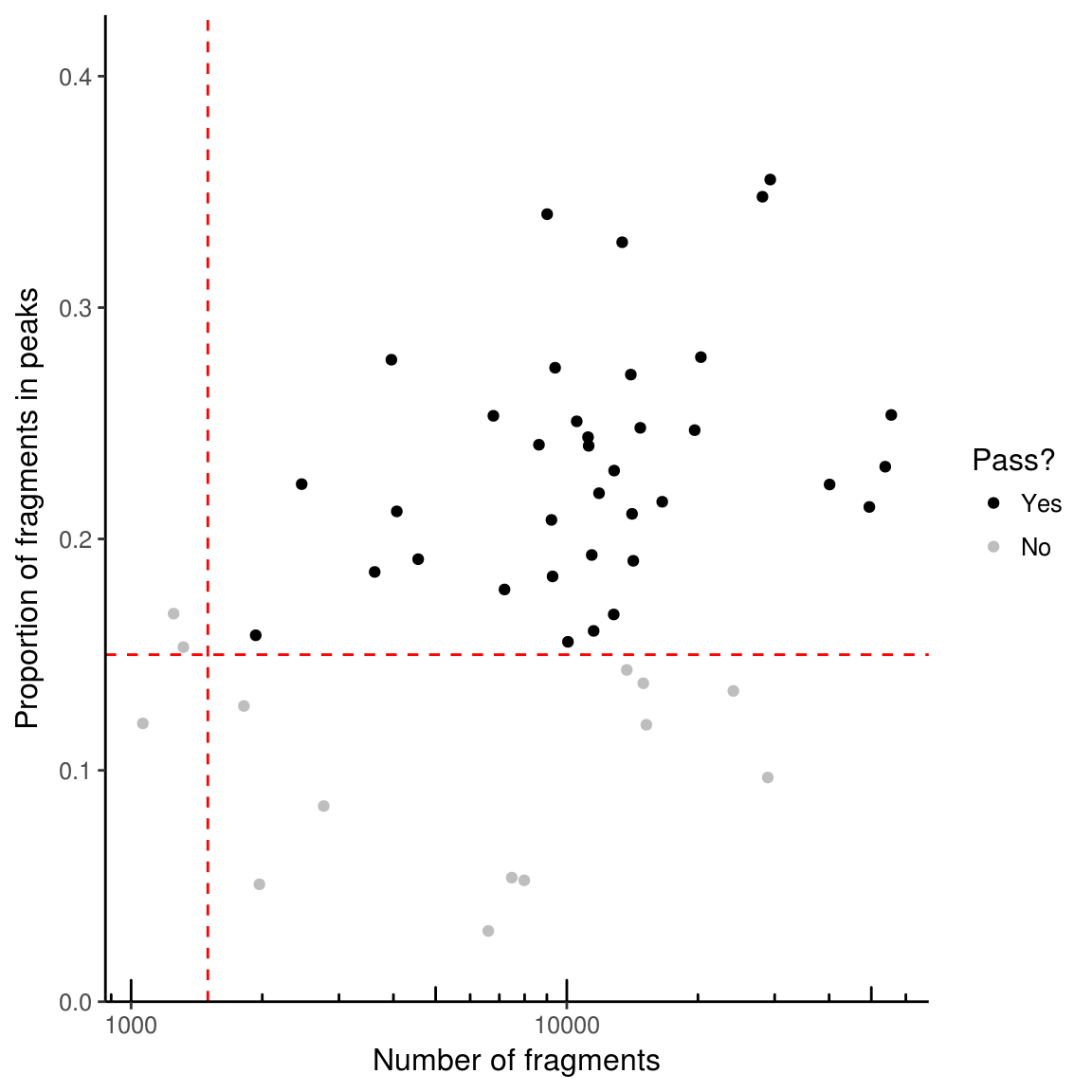
To instead return the indexes of the samples to keep instead of a new SummarizedExperiment object, use ix_return = TRUE.
ix <- filterSamples(example_counts, ix_return = TRUE, shiny = FALSE)## min_in_peaks set to 0.105## min_depth set to 1120.65Filtering peaks
For both bulk and single cell data, peaks should be filtered based on having at least a certain number of fragments. At minimum, each peak should have at least one fragment across all the samples (it might be possible to have peaks with zero reads due to using a peak set defined by other data). Otherwise, downstream functions won’t work. The function filterPeaks will also reduce the peak set to non-overlapping peaks (keeping the peak with higher counts for peaks that overlap) if non_overlapping argument is set to TRUE (which is default).
counts_filtered <- filterPeaks(counts_filtered, non_overlapping = TRUE)Session Info
Sys.Date()## [1] "2017-11-10"sessionInfo()## R Under development (unstable) (2017-11-10 r73707)
## Platform: x86_64-pc-linux-gnu (64-bit)
## Running under: Ubuntu 14.04.5 LTS
##
## Matrix products: default
## BLAS: /home/travis/R-bin/lib/R/lib/libRblas.so
## LAPACK: /home/travis/R-bin/lib/R/lib/libRlapack.so
##
## locale:
## [1] LC_CTYPE=en_US.UTF-8 LC_NUMERIC=C
## [3] LC_TIME=en_US.UTF-8 LC_COLLATE=en_US.UTF-8
## [5] LC_MONETARY=en_US.UTF-8 LC_MESSAGES=en_US.UTF-8
## [7] LC_PAPER=en_US.UTF-8 LC_NAME=C
## [9] LC_ADDRESS=C LC_TELEPHONE=C
## [11] LC_MEASUREMENT=en_US.UTF-8 LC_IDENTIFICATION=C
##
## attached base packages:
## [1] parallel stats4 methods stats graphics grDevices utils
## [8] datasets base
##
## other attached packages:
## [1] BSgenome.Hsapiens.UCSC.hg19_1.4.0 BSgenome_1.46.0
## [3] rtracklayer_1.38.0 Biostrings_2.46.0
## [5] XVector_0.18.0 Matrix_1.2-11
## [7] SummarizedExperiment_1.8.0 DelayedArray_0.4.1
## [9] matrixStats_0.52.2 Biobase_2.38.0
## [11] GenomicRanges_1.30.0 GenomeInfoDb_1.14.0
## [13] IRanges_2.12.0 S4Vectors_0.16.0
## [15] BiocGenerics_0.24.0 chromVAR_1.1.1
##
## loaded via a namespace (and not attached):
## [1] bitops_1.0-6 DirichletMultinomial_1.20.0
## [3] TFBSTools_1.16.0 bit64_0.9-7
## [5] httr_1.3.1 rprojroot_1.2
## [7] tools_3.5.0 backports_1.1.1
## [9] R6_2.2.2 DT_0.2
## [11] seqLogo_1.44.0 DBI_0.7
## [13] lazyeval_0.2.0 colorspace_1.3-2
## [15] bit_1.1-12 compiler_3.5.0
## [17] plotly_4.7.1 labeling_0.3
## [19] caTools_1.17.1 scales_0.5.0
## [21] readr_1.1.1 stringr_1.2.0
## [23] digest_0.6.12 Rsamtools_1.30.0
## [25] rmarkdown_1.7 R.utils_2.6.0
## [27] pkgconfig_2.0.1 htmltools_0.3.6
## [29] htmlwidgets_0.9 rlang_0.1.2.9000
## [31] RSQLite_2.0 VGAM_1.0-4
## [33] shiny_1.0.5 bindr_0.1
## [35] jsonlite_1.5 BiocParallel_1.12.0
## [37] gtools_3.5.0 dplyr_0.7.3
## [39] R.oo_1.21.0 RCurl_1.95-4.8
## [41] magrittr_1.5 GO.db_3.5.0
## [43] GenomeInfoDbData_0.99.1 Rcpp_0.12.13
## [45] munsell_0.4.3 R.methodsS3_1.7.1
## [47] stringi_1.1.5 yaml_2.1.14
## [49] zlibbioc_1.24.0 plyr_1.8.4
## [51] grid_3.5.0 blob_1.1.0
## [53] miniUI_0.1.1 CNEr_1.14.0
## [55] lattice_0.20-35 splines_3.5.0
## [57] annotate_1.56.0 hms_0.3
## [59] KEGGREST_1.18.0 knitr_1.17
## [61] reshape2_1.4.2 TFMPvalue_0.0.6
## [63] XML_3.98-1.9 glue_1.1.1
## [65] evaluate_0.10.1 data.table_1.10.4
## [67] png_0.1-7 httpuv_1.3.5
## [69] tidyr_0.7.1 purrr_0.2.3
## [71] gtable_0.2.0 poweRlaw_0.70.1
## [73] assertthat_0.2.0 ggplot2_2.2.1
## [75] mime_0.5 xtable_1.8-2
## [77] viridisLite_0.2.0 tibble_1.3.4
## [79] GenomicAlignments_1.14.0 AnnotationDbi_1.40.0
## [81] memoise_1.1.0 bindrcpp_0.2