chromVAR
Alicia Schep
chromVAR is an R package for the analysis of sparse chromatin accessibility. chromVAR takes as inputs aligned fragments (filtered for duplicates and low quality) from ATAC-seq or DNAse-seq experiments as well as genomic annotations such as motif positions. chromVAR computes for each annotation and each cell or sample a bias corrected “deviation” in accessibility from the expected accessibility based on the average of all the cells or samples.
This vignette covers basic usage of chromVAR with standard inputs. For more detailed documentation covering different options for various inputs and additional applications, view the additional vignettes on the documentation website. For more description of the method and applications, please see the publication (pdf, supplement).
Loading the package
Use library or require to load the package and useful additional packages.
library(chromVAR)
library(motifmatchr)
library(Matrix)
library(SummarizedExperiment)
library(BiocParallel)
set.seed(2017)
Setting multiprocessing options
The package uses BiocParallel to do the multiprocessing. Check the documentation for BiocParallel to see available options. The settings can be set using the register function. For example, to use MulticoreParam with 8 cores:
To enable progress bars for multiprocessed tasks, use
register(MulticoreParam(8, progressbar = TRUE))For Windows, MulticoreParam will not work, but you can use SnowParam:
Even if you don’t want to use more than one core, it is best to explicitly register that choice using SerialParam:
Please see the documentation for BiocParallel for more information about the register function and the various options for multi-processing.
Reading in inputs
chromVAR takes as input a table of counts of fragments falling in open chromatin peaks. There are numerous software packages that enable the creation of count tables from epigenomics data; chromVAR also provides a method that is tailored for single-cell ATAC-seq counts. To learn more about the options for the count table and how to format a count table computed via other software, see the Counts section of the documentation website.
Peaks
For using chromVAR, it is recommended to use fixed-width, non-overlapping peaks. The method is fairly robust to the exact choice of peak width, but a width of 250 to 500 bp is recommended. See the supplement of the paper for a disussion section and supplementary figures related to the choice of peak width.
If analyzing single cell data, it can make sense to use peaks derived from bulk ATAC or DNAse-seq data, either from the same population or a similar population (or possibly from a public resource, like the Roadmap Epigenomics project).
If combining multiple peak files from different populations, it is recommended to combine the peaks together. The filterPeaks function (demonstrated a bit further down this vignette) will reduce the peaks to a non-overlapping set based on which overlapping peak has stronger signal across all the data.
The function getPeaks reads in the peaks as a GenomicRanges object. We will show its use by reading in a tiny sample bed file. We’ll use the sort_peaks argument to indicate we want to sort the peaks.
peakfile <- system.file("extdata/test_bed.txt", package = "chromVAR")
peaks <- getPeaks(peakfile, sort_peaks = TRUE)
## Peaks sortedFor reading in peaks in the narrowpeak format, chromVAR includes a function, readNarrowpeaks, that will read in the file, resize the peaks to a given size based on the width argument, and remove peaks that overlap a peak with stronger signal (if non_overlapping is set to TRUE – the default).
Counts
The function getCounts returns a chromVARCounts object with a Matrix of fragment counts per sample/cell for each peak in assays. This data can be accessed with counts(fragment_counts).The Matrix package is used so that if the matrix is sparse, the matrix will be stored as a sparse Matrix. We will demonstrate this function with a very tiny set of reads included in the package:
bamfile <- system.file("extdata/test_RG.bam", package = "chromVAR")
fragment_counts <- getCounts(bamfile,
                             peaks,
                             paired =  TRUE,
                             by_rg = TRUE,
                             format = "bam",
                             colData = DataFrame(celltype = "GM"))
## Reading in file: /home/travis/R/Library/chromVAR/extdata/test_RG.bam## Warning in doTryCatch(return(expr), name, parentenv, handler): length of
## NULL cannot be changedHere we passed only one bam file, but we can also pass a vector of bam file names. In that case, for the column data we would specify the appropriate value per file, e.g DataFrame(celltype = c("GM","K562")) if we were passing in one file for GM cells and one for K562 cells.
If RG tags are not used for combining multiple samples within a file, use by_rg = FALSE. For more on reading in counts, see the Counts section of the documentation website.
Example data
For the rest of the vignette, we will use a very small (but slightly larger than the previous example) data set of 10 GM cells and 10 H1 cells that has already been read in as a SummarizedExperiment object.
data(example_counts, package = "chromVAR")
head(example_counts)
## class: RangedSummarizedExperiment
## dim: 6 50
## metadata(0):
## assays(1): counts
## rownames: NULL
## rowData names(3): score qval name
## colnames(50): singles-GM12878-140905-1 singles-GM12878-140905-2
## ... singles-H1ESC-140820-24 singles-H1ESC-140820-25
## colData names(2): Cell_Type depthGetting GC content of peaks
The GC content will be used for determining background peaks. The function addGCBias returns an updated SummarizedExperiment with a new rowData column named “bias”. The function requires an input of a genome sequence, which can be provided as a BSgenome, FaFile, or DNAStringSet object.
library(BSgenome.Hsapiens.UCSC.hg19)
example_counts <- addGCBias(example_counts,
                            genome = BSgenome.Hsapiens.UCSC.hg19)
head(rowData(example_counts))
## DataFrame with 6 rows and 4 columns
## score qval name bias
## <integer> <numeric> <character> <numeric>
## 1 259 25.99629 GM_peak_6 0.652
## 2 82 8.21494 H1_peak_7 0.680
## 3 156 15.65456 GM_peak_17 0.788
## 4 82 8.21494 H1_peak_13 0.674
## 5 140 14.03065 GM_peak_27 0.600
## 6 189 18.99529 GM_peak_29a 0.742Check out available.genomes from the BSgenome package for what genomes are available as BSgenome packages. For making your own BSgenome object, check out BSgenomeForge.
Filtering inputs
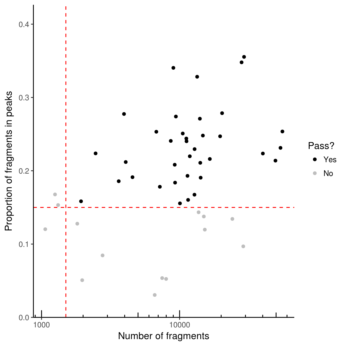
If working with single cell data, it is advisable to filter out samples with insufficient reads or a low proportion of reads in peaks as these may represent empty wells or dead cells. Two parameters are used for filtering – min_in_peaks and min_depth. If not provided (as above), these cutoffs are estimated based on the medians from the data. min_in_peaks is set to 0.5 times the median proportion of fragments in peaks. min_depth is set to the maximum of 500 or 10% of the median library size.
Unless plot = FALSE given as argument to function filterSamples, a plot will be generated.
#find indices of samples to keep
counts_filtered <- filterSamples(example_counts, min_depth = 1500,
                                 min_in_peaks = 0.15, shiny = FALSE)
If shiny argument is set to TRUE (the default), a shiny gadget will pop up which allows you to play with the filtering parameters and see which cells pass filters or not.
To get just the plot of what is filtered, use filterSamplesPlot. By default, the plot is interactive– to set it as not interactive use use_plotly = FALSE.
#find indices of samples to keep
filtering_plot <- filterSamplesPlot(example_counts, min_depth = 1500,
                                    min_in_peaks = 0.15, use_plotly = FALSE)
filtering_plot
To instead return the indexes of the samples to keep instead of a new SummarizedExperiment object, use ix_return = TRUE.
ix <- filterSamples(example_counts, ix_return = TRUE, shiny = FALSE)## min_in_peaks set to 0.105## min_depth set to 1120.65For both bulk and single cell data, peaks should be filtered based on having at least a certain number of fragments. At minimum, each peak should have at least one fragment across all the samples (it might be possible to have peaks with zero reads due to using a peak set defined by other data). Otherwise, downstream functions won’t work. The function filterPeaks will also reduce the peak set to non-overlapping peaks (keeping the peak with higher counts for peaks that overlap) if non_overlapping argument is set to TRUE (which is the default).
counts_filtered <- filterPeaks(counts_filtered, non_overlapping = TRUE)Get motifs and what peaks contain motifs
The function getJasparMotifs fetches motifs from the JASPAR database.
motifs <- getJasparMotifs()The function getJasparMotifs() by default gets human motifs from JASPAR core database. For other species motifs, change the species argument.
yeast_motifs <- getJasparMotifs(species = "Saccharomyces cerevisiae")For using a collection other than core, use the collection argument. Options include: “CORE”, “CNE”, “PHYLOFACTS”, “SPLICE”, “POLII”, “FAM”, “PBM”, “PBM_HOMEO”, “PBM_HLH”.
The getJasparMotifs function is simply a wrapper around getMatrixSet from TFBSTools– you can also use that function to fetch motifs from JASPAR if you prefer, and/or check out the documentation for that function for more information.
The function matchMotifs from the motifmatchr package finds which peaks contain which motifs. By default, it returns a SummarizedExperiment object, which contains a sparse matrix indicating motif match or not.The function requires an input of a genome sequence, which can be provided as a BSgenome, FaFile, or DNAStringSet object.
library(motifmatchr)
motif_ix <- matchMotifs(motifs, counts_filtered,
                        genome = BSgenome.Hsapiens.UCSC.hg19)
One option is the p.cutoff for determing how stringent motif calling should be. The default value is 0.00005, which tends to give reasonable numbers of motif matches for human motifs.
Instead of returning just motif matches, the function can also return additional matrices (stored as assays) with the number of motif matches per peak and the maximum motif score per peak. For this additional information, use out = scores. To return the actual positions of motif matches, use out = positions. Either the output with out = matches or out = scores can be passed to the computeDeviations function.
If instead of using known motifs, you want to use all kmers of a certain length, the matchKmers function can be used. For more about using kmers as inputs, see the the Annotations section of the documentation website.
kmer_ix <- matchKmers(6, counts_filtered,
                      genome = BSgenome.Hsapiens.UCSC.hg19)
Compute deviations
The function computeDeviations returns a SummarizedExperiment with two “assays”. The first matrix (accessible via deviations(dev) or assays(dev)$deviations) will give the bias corrected “deviation” in accessibility for each set of peaks (rows) for each cell or sample (columns). This metric represent how accessible the set of peaks is relative to the expectation based on equal chromatin accessibility profiles across cells/samples, normalized by a set of background peak sets matched for GC and average accessability. The second matrix (deviationScores(dev) or assays(deviations)$z) gives the deviation Z-score, which takes into account how likely such a score would occur if randomly sampling sets of beaks with similar GC content and average accessibility.
dev <- computeDeviations(object = counts_filtered, annotations = motif_ix)Background Peaks
The function computeDeviations will use a set of background peaks for normalizing the deviation scores. This computation is done internally by default and not returned – to have greater control over this step, a user can run the getBackgroundPeaks function themselves and pass the result to computeDeviations under the background_peaks parameter.
Background peaks are peaks that are similar to a peak in GC content and average accessibility.
bg <- getBackgroundPeaks(object = counts_filtered)The result from getBackgroundPeaks is a matrix of indices, where each column represents the index of the peak that is a background peak.
To use the background peaks computed, simply add those to the call to computeDeviations:
dev <- computeDeviations(object = counts_filtered, annotations = motif_ix,
                         background_peaks = bg)
Variability
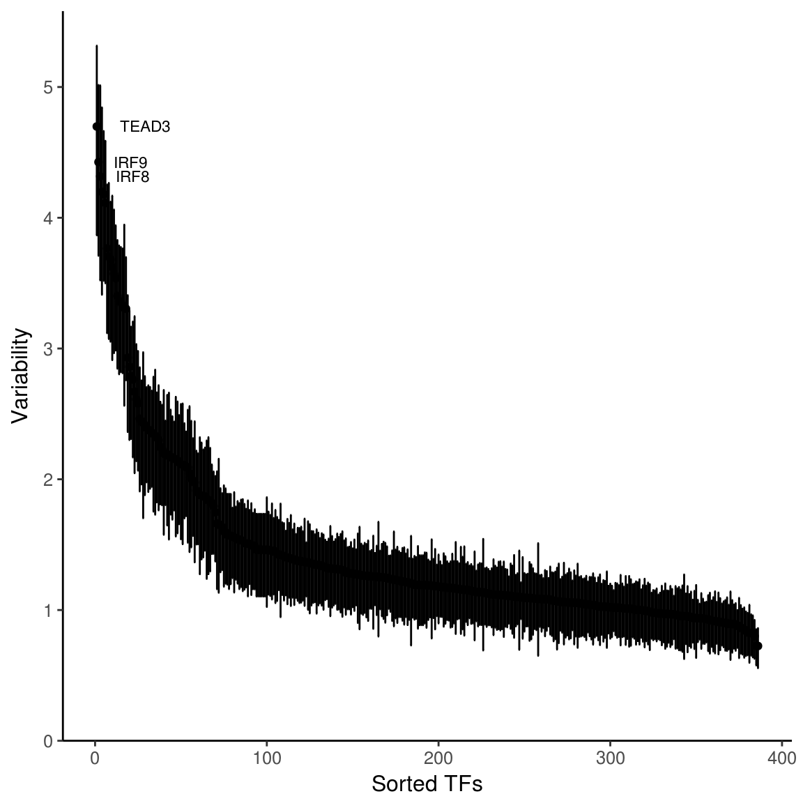
The function computeVariability returns a data.frame that contains the variability (standard deviation of the z scores computed above across all cell/samples for a set of peaks), bootstrap confidence intervals for that variability (by resampling cells/samples), and a p-value for the variability being greater than the null hypothesis of 1.
variability <- computeVariability(dev)

plotVariability(variability, use_plotly = FALSE) 
plotVariability takes the output of computeVariability and returns a plot of rank sorted annotation sets and their variability. By default, the plot will be interactive, unless you set use_plotly = FALSE.
Visualizing Deviations
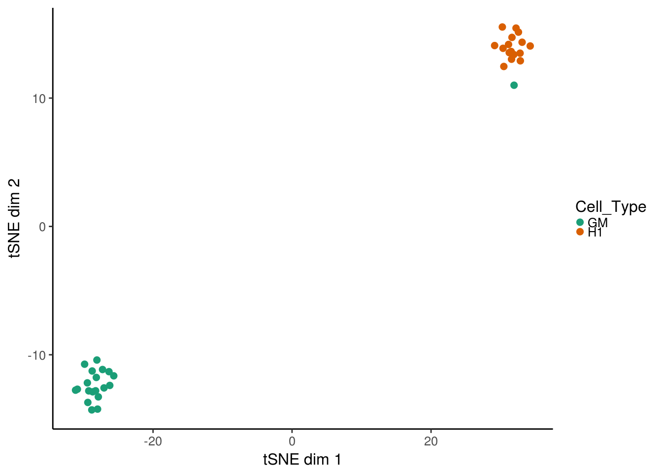
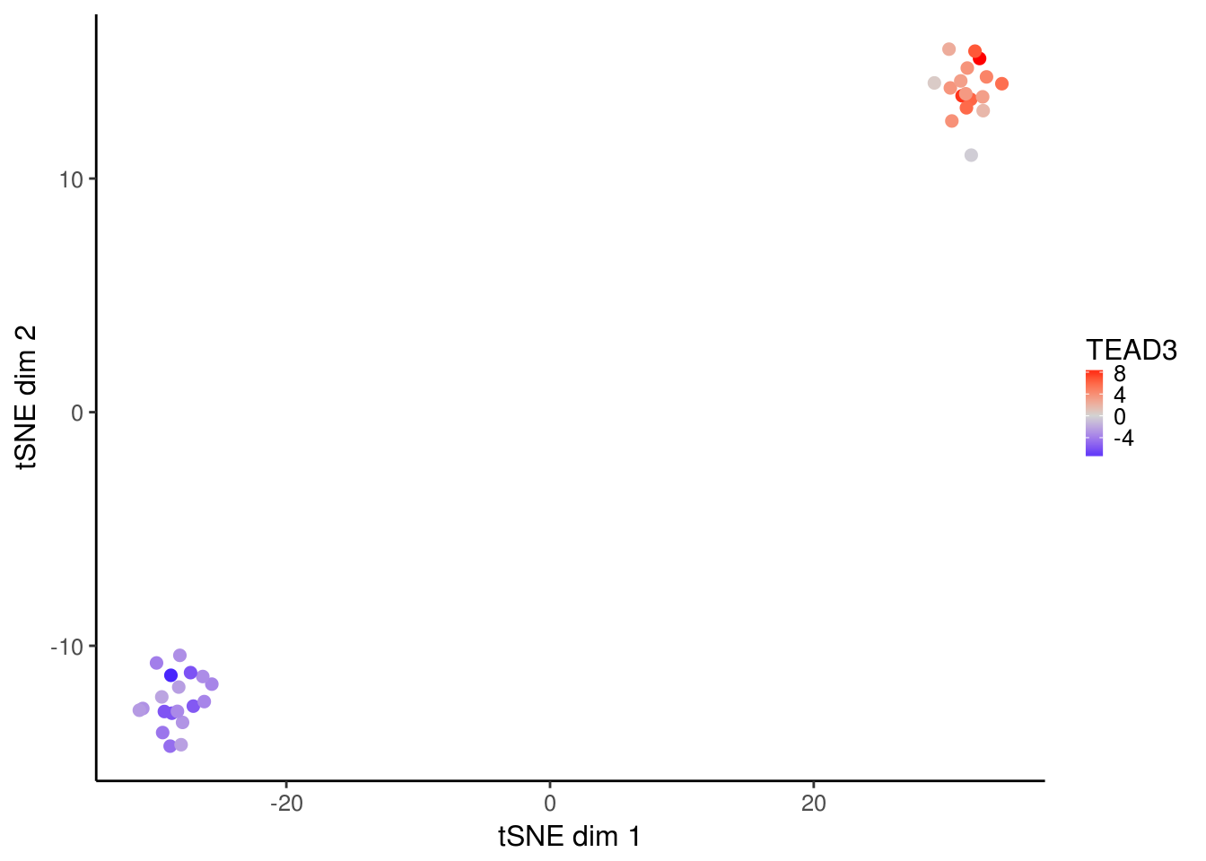
For visualizing cells, it can be useful to project the deviation values into two dimension using TSNE. A convenience function for doing so is provided in deviationsTsne. If running in an interactive session, shiny can be set to TRUE to load up a shiny gadget for exploring parameters.
tsne_results <- deviationsTsne(dev, threshold = 1.5, perplexity = 10)To plot the results, plotDeviationsTsne can be used. If running in an interactive session or an interactive Rmarkdown document, shiny can be set to TRUE to generate a shiny widget. Here we will show static results.
tsne_plots <- plotDeviationsTsne(dev, tsne_results,
                                 annotation_name = "TEAD3",
                                   sample_column = "Cell_Type",
                                 shiny = FALSE)
tsne_plots[[1]]
tsne_plots[[2]]
Session Info
Sys.Date()## [1] "2017-11-10"sessionInfo()## R Under development (unstable) (2017-11-10 r73707)
## Platform: x86_64-pc-linux-gnu (64-bit)
## Running under: Ubuntu 14.04.5 LTS
##
## Matrix products: default
## BLAS: /home/travis/R-bin/lib/R/lib/libRblas.so
## LAPACK: /home/travis/R-bin/lib/R/lib/libRlapack.so
##
## locale:
## [1] LC_CTYPE=en_US.UTF-8 LC_NUMERIC=C
## [3] LC_TIME=en_US.UTF-8 LC_COLLATE=en_US.UTF-8
## [5] LC_MONETARY=en_US.UTF-8 LC_MESSAGES=en_US.UTF-8
## [7] LC_PAPER=en_US.UTF-8 LC_NAME=C
## [9] LC_ADDRESS=C LC_TELEPHONE=C
## [11] LC_MEASUREMENT=en_US.UTF-8 LC_IDENTIFICATION=C
##
## attached base packages:
## [1] parallel stats4 methods stats graphics grDevices utils
## [8] datasets base
##
## other attached packages:
## [1] BSgenome.Hsapiens.UCSC.hg19_1.4.0 BSgenome_1.46.0
## [3] rtracklayer_1.38.0 Biostrings_2.46.0
## [5] XVector_0.18.0 BiocParallel_1.12.0
## [7] SummarizedExperiment_1.8.0 DelayedArray_0.4.1
## [9] matrixStats_0.52.2 Biobase_2.38.0
## [11] GenomicRanges_1.30.0 GenomeInfoDb_1.14.0
## [13] IRanges_2.12.0 S4Vectors_0.16.0
## [15] BiocGenerics_0.24.0 Matrix_1.2-11
## [17] motifmatchr_1.1.1 chromVAR_1.1.1
##
## loaded via a namespace (and not attached):
## [1] bitops_1.0-6 DirichletMultinomial_1.20.0
## [3] TFBSTools_1.16.0 bit64_0.9-7
## [5] RColorBrewer_1.1-2 httr_1.3.1
## [7] rprojroot_1.2 tools_3.5.0
## [9] backports_1.1.1 R6_2.2.2
## [11] DT_0.2 seqLogo_1.44.0
## [13] DBI_0.7 lazyeval_0.2.0
## [15] colorspace_1.3-2 bit_1.1-12
## [17] compiler_3.5.0 plotly_4.7.1
## [19] labeling_0.3 caTools_1.17.1
## [21] scales_0.5.0 readr_1.1.1
## [23] nabor_0.4.7 stringr_1.2.0
## [25] digest_0.6.12 Rsamtools_1.30.0
## [27] rmarkdown_1.7 R.utils_2.6.0
## [29] pkgconfig_2.0.1 htmltools_0.3.6
## [31] htmlwidgets_0.9 rlang_0.1.2.9000
## [33] RSQLite_2.0 VGAM_1.0-4
## [35] shiny_1.0.5 bindr_0.1
## [37] jsonlite_1.5 gtools_3.5.0
## [39] dplyr_0.7.3 R.oo_1.21.0
## [41] RCurl_1.95-4.8 magrittr_1.5
## [43] GO.db_3.5.0 GenomeInfoDbData_0.99.1
## [45] Rcpp_0.12.13 munsell_0.4.3
## [47] R.methodsS3_1.7.1 stringi_1.1.5
## [49] yaml_2.1.14 zlibbioc_1.24.0
## [51] Rtsne_0.13 plyr_1.8.4
## [53] grid_3.5.0 blob_1.1.0
## [55] miniUI_0.1.1 CNEr_1.14.0
## [57] lattice_0.20-35 splines_3.5.0
## [59] annotate_1.56.0 hms_0.3
## [61] KEGGREST_1.18.0 knitr_1.17
## [63] JASPAR2016_1.6.0 codetools_0.2-15
## [65] reshape2_1.4.2 TFMPvalue_0.0.6
## [67] XML_3.98-1.9 glue_1.1.1
## [69] evaluate_0.10.1 data.table_1.10.4
## [71] png_0.1-7 httpuv_1.3.5
## [73] tidyr_0.7.1 purrr_0.2.3
## [75] gtable_0.2.0 poweRlaw_0.70.1
## [77] assertthat_0.2.0 ggplot2_2.2.1
## [79] mime_0.5 xtable_1.8-2
## [81] viridisLite_0.2.0 tibble_1.3.4
## [83] GenomicAlignments_1.14.0 AnnotationDbi_1.40.0
## [85] memoise_1.1.0 bindrcpp_0.2